MANE 6313
Week 12, Module A
Student Learning Outcome
- Select an appropriate experimental design with one or more factors,
- Select an appropriate model with one or more factors,
- Evaluate statistical analyses of experimental designs,
- Assess the model adequacy of any experimental design, and
- Interpret model results.
Module Learning Outcome
Describe linear regression.
Resources for the Week 12, Module A micro-lecture are:
Introduction to Linear Regression
-
We are interested in a relationship between a single dependent variable or response \(y\) that depends on \(k\) independent or regressor variables.
-
We assume that there is some mathematical function \(y=\phi(x_1,x_2,\ldots,x_k)\). In general, we don't know this function
-
We'll use low order polynomial equations as an approximating function. This is called empirical modeling.
-
What are methods that we can determine if there is a relationship between two (or more) variables?
Relationship between two or more variables
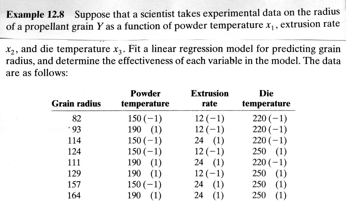
Example is from Walpole, Meyers and Meyers (1998)1
Linear regression models
- In general they look like
- This model is linear in the parameters \(\beta\)
- See graphical explanation from Ott.
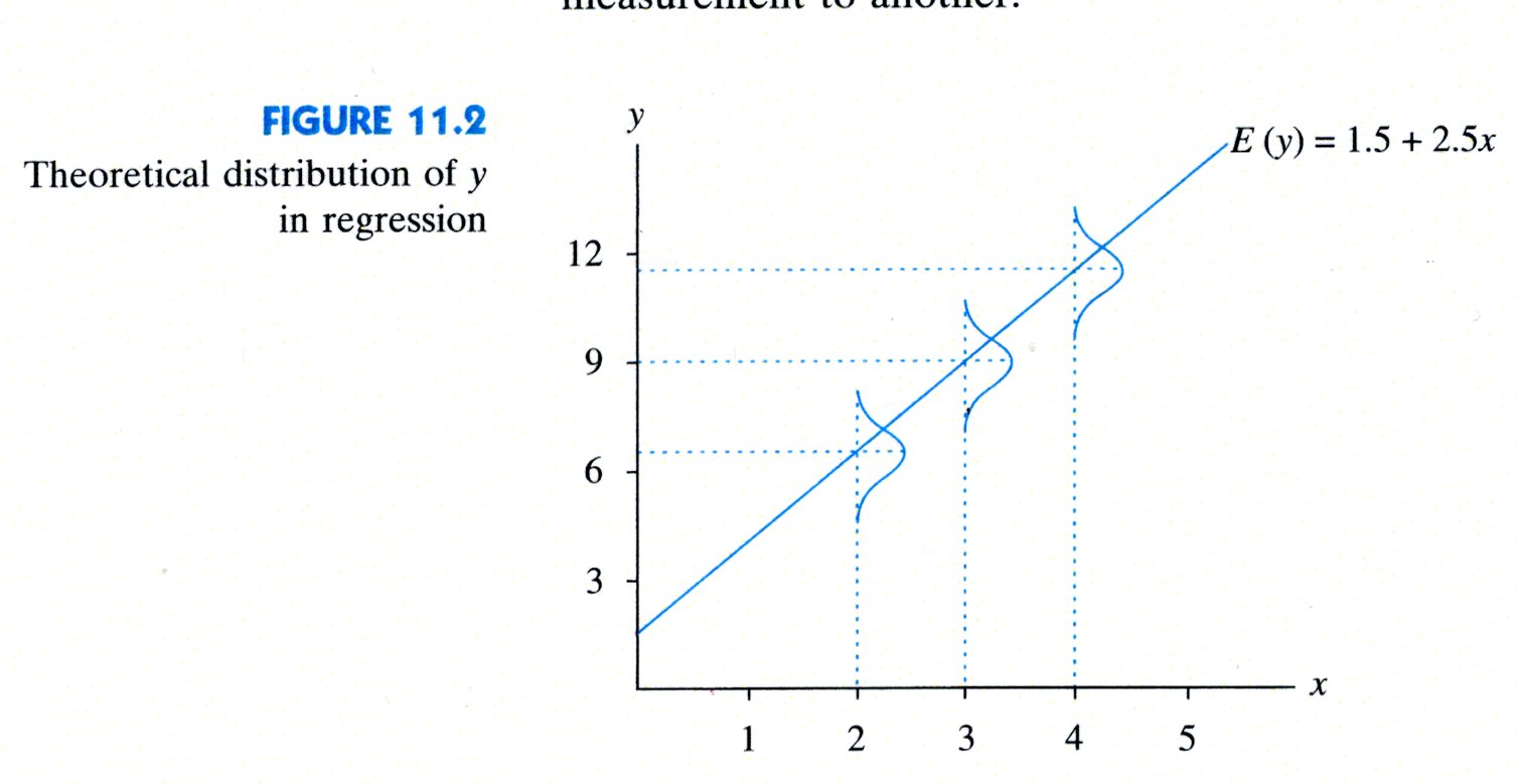
Taken from Longnecker and Ott (2001)2
Estimation of Parameters
- Parameter estimates are derived using least squares. Goal is to minimize the squared error.
- In general, the matrix formulation is used. Model is defined to be
- The least squares estimates are found by minimizing
- The least squares estimates must satisfy
- Which leads to the solution
- We can define the predicted response to be
- The residuals are defined to be
- Thus the sum of squares errors can be shown to be
Matrix Formulation Example
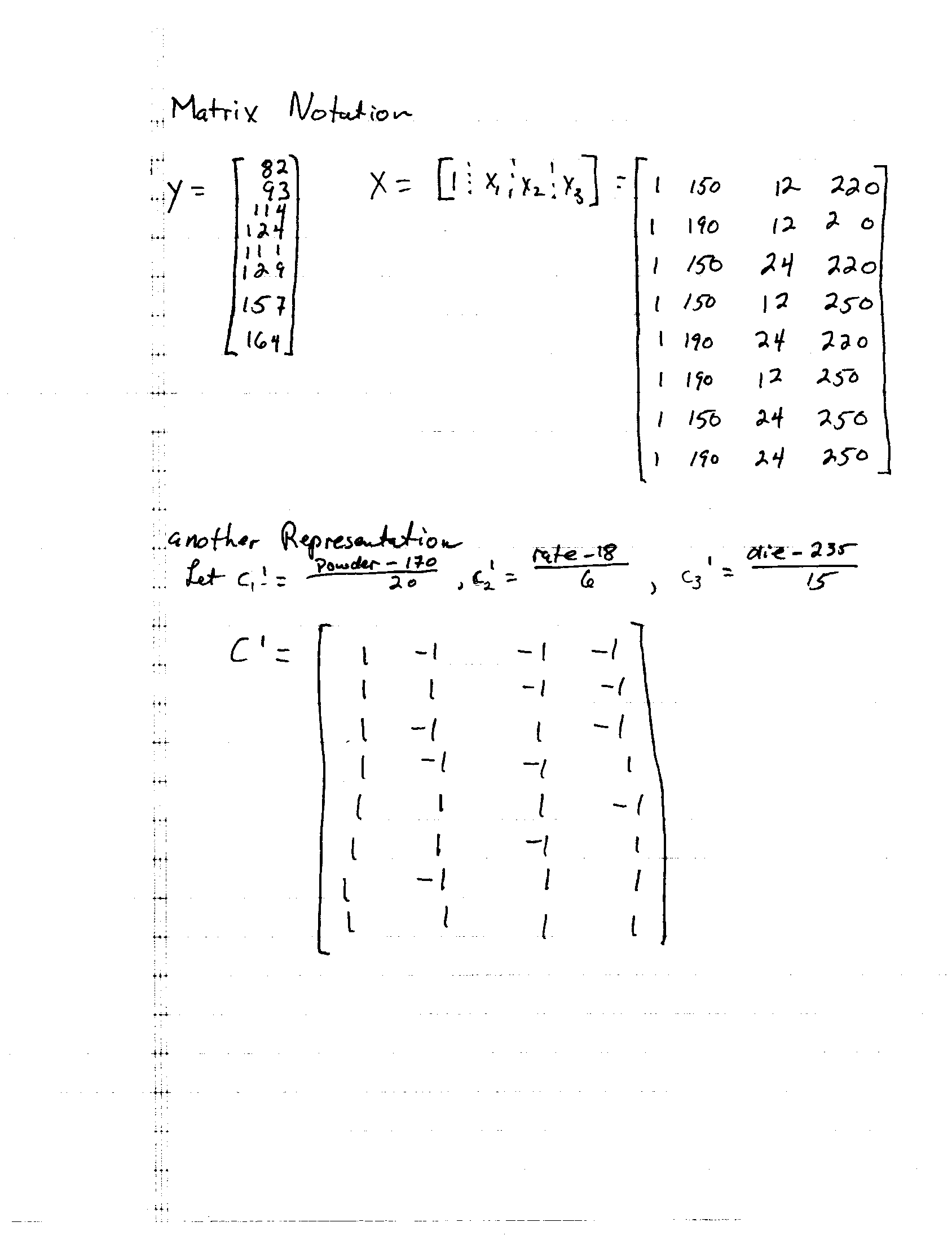
Coding Variables
-
From the example, there were two ways to represent the same problem, coded and uncoded
-
Why use coded variables3
-
Computational ease and increased accuracy in estimating the model coefficients
-
Enhanced interpretability of the coefficient estimates in the model.
-
-
Internally most statistical software codes for estimating parameters
-
Walpole, Myers, and Myers (1998). Probability and Statistics for Engineers and Scientists, 6th edition. Prentice-Hall. ↩
-
Longnecker and Ott (2001). An Introduction to Statistical Methods and Data Analysis, 5th edition. Duxbury. ↩
-
Khuri, and Cornell (1987). Response Surfaces: Designs and Analyses. Dekker ↩