MANE 3351
Lecture 12, September 29
Classroom Management
Agenda
- Lab today in ENGR 2.268 at 3:30 pm
- GitHub Accounts
- Sign up for free student GitHub account at https://education.github.com/students
- Register your student GitHub account with MANE 3351 GitHub classroom email
- Lecture
Resources
Handouts
- Lecture 12 Slides
- Lecture 12 Marked Slides
Calendar
| Lecture | Date | Content |
|---|---|---|
| 1 | August 23 | Welcome to Class, Syllabus |
| 2 | August 25 | Error Analysis |
| 3 | August 30 | Introduction to Jupyter Notebook |
| 4 | September 1 | Markdown |
| 5 | September 6 | Labor Day Holiday |
| 6 | September 8 | Taylor Polynomials, Homework 1 |
| 7 | September 13 | Roots of Equations, Bisection Method |
| 8 | September 15 | Bisection Error Analysis |
| 9 | September 20 | False Position Algorithm |
| 10 | September 22 | Newton Raphson Algorithm |
| 11 | September 27 | Secant Method |
| 12 | September 29 | Numerical Integration |
Assignments
- Homework 3 (assigned 9/22/2021, due 9/30/2021)
Looking Ahead
| Lecture | Date | Content |
|---|---|---|
| 13 | October 4 | Simpson's Rule |
| 14 | October 6 | Romberg Integration |
| 15 | October 11 | Gaussian Quadrature (end of material for Test 1) |
| 16 | October 13 | Vectors |
| 17 | October 18 | Vector Operations |
| 18 | October 20 | Test 1 |
Lecture 12, September 29
Today's topic is numerical integration. This is a major new topic after root finding.
Introduction
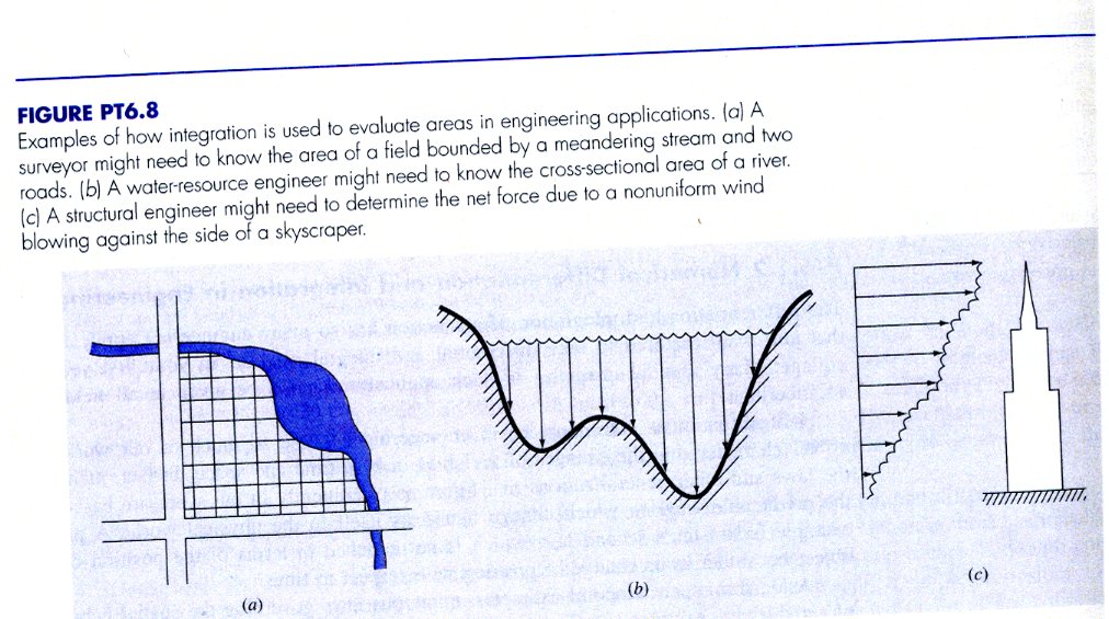
- In layman's terms, an integral calculates the area under a curve
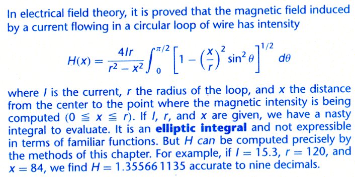
- Frequently used in engineering analysis
Definitions
Cheney and Kincaid (2004)1 provide the following definitions
- Indefinite integral : \(\int x^2\;dx=\frac{1}{3}x^3+C\)
- Definite integral: \(\int x^2\; dx = \frac{8}{3}\)
Numerical Integration
Kiusalaas (2013)2 suggest three major approaches to numerical integration that we will investigate:
- Newton-Cotes
a. Trapezoid rule (n=1)
b. Simpson's rule (n=2)
c. 3/8 Simpson's rule (n=3)
-
Romberg Integration
-
Gaussian Quadrature
Note: there are many different techniques for numerical integration than the ones listed above
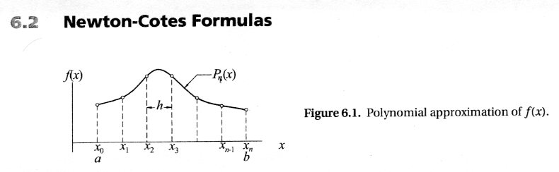
Newton-Cotes Formulas
Kiusalass (2013)2 provide the following illustration to explain Newton-Cotes techniques
Trapezoid Rule
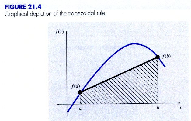
Chapra and Canale (2015)3 provide the figure shown below illustrating the trapezoid rule
Trapezoid Rule, continued
Chapra and Canale (2015)3 provided the following formulae
- \(I=(b-a)\frac{f(a)+f(b)}{2}\)
- \(E=-\frac{1}{12}f^{\prime\prime}\left(\xi\right)\left(b-a\right)^3\)
Multiple Applications of the Trapezoid Rule
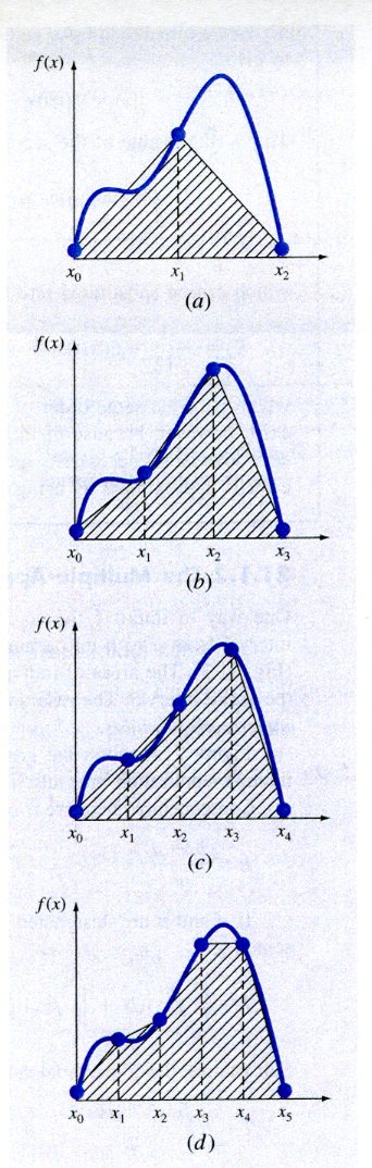
Typically, the region form \(a\) to \(b\) is sub-divided into multiple regions and then the Trapezoid Rule for each region is applied. Chapra and Canale (2015)3 illustrate this concept.
Uniform Spacing
Cheney and Kincaid (2004)1 the following formula for composite (multiple) applications of the Trapezoid Rule $$ \int_a^b=f(x)dx\approx T(f;P)=h\left{\sum_{i=1}^{n-1}f\left(x_i\right)+\frac{1}{2}\left[f\left(x_0\right)+f\left(x_n\right)\right]\right} $$
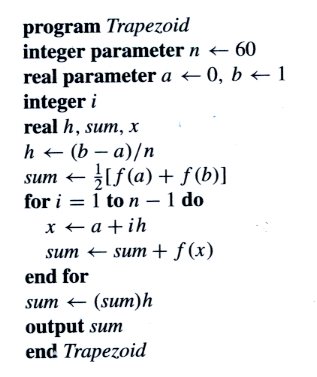
Pseudo-code
Cheney and Kincaid (2004)1 provided the following pseudo-code for the composite trapezoid rule